Table of Contents
Dispersion function documentation for the xrays RF Ray tracing code.
Introduction
This page documents the types of dispersion functions available. As a ray moves through the plasma it must remain a solution of these functions. For a fixed wave frequency \(\omega \), the dispersion function dictates how the wave number \(\vec{k}\) and ray trajectory \(\vec{x}\) interact.
| Symbol | Unit | Description |
|---|---|---|
| \(c \) | \(\frac{m}{s}\) | Speed of light. |
| \(m_{e}\) | \(kg \) | Electron mass |
| \(t_{e}\) | \(K \) | Electron temperature |
| \(n_{e}\) | \(m^{-3}\) | Electron Density |
| \(q \) | \(C \) | Fundamental Charge |
| \(\vec{B}\) | \(T \) | Magnetic field |
| \(\epsilon_{0}\) | \(\frac{F}{m}\) | Vacuum permittivity |
| \(k_{B}\) | \(\frac{J}{K}\) | Boltzmann constant |
| \(\omega_{pe}\) | \(s^{-1}\) | Electron Plasma Frequency \(\omega_{pe}=\frac{n_{e}q^{2}}{\epsilon_{0}m_{e}c}\) |
| \(\omega_{ce}\) | \(s^{-1}\) | Electron Cyclotron Frequency \(\omega_{ce}=\frac{q\left|\vec{B}\right|}{m_{e}}\) |
| \(\omega_{h}\) | \(s^{-1}\) | Upper Hybrid Frequency \(\omega_{h}^{s}=\omega_{pe}^{2}+\omega_{ce}^{2}\) |
| \(\omega_{r}\) | \(s^{-1}\) | Right cutoff Frequency \(\omega_{r}=\frac{1}{2}\left(\omega_{ce}+\sqrt{\omega^{2}_{ce}+4\omega_{pe}^{2}}\right)\) |
| \(\omega_{l}\) | \(s^{-1}\) | Left cutoff Frequency \(\omega_{r}=\frac{1}{2}\left(-\omega_{ce}+\sqrt{\omega^{2}_{ce}+4\omega_{pe}^{2}}\right)\) |
| \(v_{th}\) | \(\frac{m}{s}\) | Thermal velocity \(v_{th}=\sqrt{\frac{k_{B}t_{e}}{m_{e}}}\) |
| \(\vec{n}\) | \(1 \) | \(n=\frac{\vec{k}c}{\omega}\) |
Normalization
The dispersion functions use normalized quantities for frequency \(\omega \) and time \(t \). These are scaled to the speed of light \(c \).
| Symbol | Real Unit | Modified | Modified Unit | Description |
|---|---|---|---|---|
| \(\omega \) | \(s^{-1}\) | \(\omega'=\frac{\omega}{c}\) | \(m^{-1}\) | Wave frequency |
| \(\vec{k}\) | \(m^{-1}\) | \(\vec{k}\) | \(m^{-1}\) | Wave number |
| \(t \) | \(s \) | \(t'=tc \) | \(m \) | Time |
| \(\vec{x}\) | \(m \) | \(\vec{x}\) | \(m \) | Position |
| \(v_{p}=\frac{\omega}{k}\) | \(\frac{m}{s}\) | \(v'_{p}=\frac{\omega'}{k}\) | \(1 \) | Phase velocity |
| \(v_{g}=\frac{\partial\omega}{\partial k}\) | \(\frac{m}{s}\) | \(v'_{g}=\frac{\partial\omega'}{\partial k}\) | \(1 \) | Group velocity |
Wave propagation
From any dispersion function, the wave propagation equations are obtained from derivatives of the dispersion relation.
\begin{equation}\frac{\partial\vec{x}}{\partial {t}}=-\frac{\frac{\partial D\left(\omega,\vec{k},\vec{x}\right)}{\partial\vec{k}}}{\frac{\partial D\left(\omega,\vec{k},\vec{x}\right)}{\partial\omega}}\end{equation}
\begin{equation}\frac{\partial\vec{k}}{\partial {t}}=\frac{\frac{\partial D\left(\omega,\vec{k},\vec{x}\right)}{\partial\vec{x}}}{\frac{\partial D\left(\omega,\vec{k},\vec{x}\right)}{\partial\omega}}\end{equation}
RF waves are traced by integrating this system of equations.
Generalized to arbitrary coordinates
This section works through the math for generalizing the ray equations to generalized coordinates. This is needed for working in non-normalized, non-orthogonal coordinate systems like those used in stellarator equilibrium. A point in 3D space can be defined in a flux coordinate system \(\vec{x}\left(s,u,v\right)\). From here a set of covariant basis vector can be defined.
\begin{equation}\vec{e}_{s}=\frac{\partial \vec{x}}{\partial s}\end{equation}
\begin{equation}\vec{e}_{u}=\frac{\partial \vec{x}}{\partial u}\end{equation}
\begin{equation}\vec{e}_{v}=\frac{\partial \vec{x}}{\partial v}\end{equation}
From this basis set, we can defined a coordinate system Jacobian \(\mathcal{J}=\vec{e}_{s}\cdot\vec{e}_{u}\times\vec{e}_{v}\). Using this the reciprocal (contravariant) basis set is defined as
\begin{equation}\vec{e}^{s}=\frac{\vec{e}_{u}\times\vec{e}_{v}}{\mathcal{J}}\end{equation}
\begin{equation}\vec{e}^{u}=\frac{\vec{e}_{v}\times\vec{e}_{s}}{\mathcal{J}}\end{equation}
\begin{equation}\vec{e}^{v}=\frac{\vec{e}_{s}\times\vec{e}_{u}}{\mathcal{J}}\end{equation}
Any vector such as the wave number \(\vec{k}\) can be written in either basis.
\begin{equation}\vec{k}=k^{s}\vec{e}_{s}+k^{u}\vec{e}_{u}+k^{v}\vec{e}_{v}=k_{s}\vec{e}^{s}+k_{u}\vec{e}^{u}+k_{v}\vec{e}^{v}\end{equation}
We now need to write our wave propagation equations in terms of the basis vectors. The left hand sides can be expanded to.
\begin{equation}\frac{\partial\vec{x}}{\partial {t}}=\frac{\partial s}{\partial t}\frac{\partial\vec{x}}{\partial s}+\frac{\partial u}{\partial t}\frac{\partial\vec{x}}{\partial u}+\frac{\partial v}{\partial t}\frac{\partial\vec{x}}{\partial v}=\frac{\partial s}{\partial t}\vec{e}_{s}+\frac{\partial u}{\partial t}\vec{e}_{u}+\frac{\partial v}{\partial t}\vec{e}_{v}\end{equation}
\begin{equation}\frac{\partial\vec{k}}{\partial {t}}=\frac{\partial k_{s}}{\partial t}\frac{\partial \vec{k}}{\partial k_{s}}+\frac{\partial k_{u}}{\partial t}\frac{\partial \vec{k}}{\partial k_{u}}+\frac{\partial k_{v}}{\partial t}\frac{\partial \vec{k}}{\partial k_{v}}=\frac{\partial k_{s}}{\partial t}\vec{e}^{s}+\frac{\partial k_{u}}{\partial t}\vec{e}^{u}+\frac{\partial k_{v}}{\partial t}\vec{e}^{v}\end{equation}
We now need to write the righthand side in terms of the covariant and contravariant basis sets. Ignoring the scalar quantity in the denominator,
\begin{equation}\frac{\partial D\left(\omega,\vec{k},\vec{x}\right)}{\partial k_{s}}=\frac{\partial D\left(\omega,\vec{k},\vec{x}\right)}{\partial\vec{k}}\frac{\partial\vec{k}}{\partial k_{s}}=\frac{\partial D\left(\omega,\vec{k},\vec{x}\right)}{\partial\vec{k}}\vec{e}^{s}\end{equation}
\begin{equation}\frac{\partial D\left(\omega,\vec{k},\vec{x}\right)}{\partial k_{u}}=\frac{\partial D\left(\omega,\vec{k},\vec{x}\right)}{\partial\vec{k}}\frac{\partial\vec{k}}{\partial k_{u}}=\frac{\partial D\left(\omega,\vec{k},\vec{x}\right)}{\partial\vec{k}}\vec{e}^{u}\end{equation}
\begin{equation}\frac{\partial D\left(\omega,\vec{k},\vec{x}\right)}{\partial k_{v}}=\frac{\partial D\left(\omega,\vec{k},\vec{x}\right)}{\partial\vec{k}}\frac{\partial\vec{k}}{\partial k_{v}}=\frac{\partial D\left(\omega,\vec{k},\vec{x}\right)}{\partial\vec{k}}\vec{e}^{v}\end{equation}
Noting that \(\vec{e}^{i}\cdot\vec{e}_{j}=\delta^{i}_{j}\)
\begin{equation}\frac{\partial D\left(\omega,\vec{k},\vec{x}\right)}{\partial k_{s}}\vec{e}_{s}=\frac{\partial D\left(\omega,\vec{k},\vec{x}\right)}{\partial\vec{k}}\vec{e}^{s}\cdot\vec{e}_{s}=\frac{\partial D\left(\omega,\vec{k},\vec{x}\right)}{\partial\vec{k}}\end{equation}
\begin{equation}\frac{\partial D\left(\omega,\vec{k},\vec{x}\right)}{\partial k_{u}}\vec{e}_{u}=\frac{\partial D\left(\omega,\vec{k},\vec{x}\right)}{\partial\vec{k}}\vec{e}^{u}\cdot\vec{e}_{u}=\frac{\partial D\left(\omega,\vec{k},\vec{x}\right)}{\partial\vec{k}}\end{equation}
\begin{equation}\frac{\partial D\left(\omega,\vec{k},\vec{x}\right)}{\partial k_{v}}\vec{e}_{v}=\frac{\partial D\left(\omega,\vec{k},\vec{x}\right)}{\partial\vec{k}}\vec{e}^{v}\cdot\vec{e}_{v}=\frac{\partial D\left(\omega,\vec{k},\vec{x}\right)}{\partial\vec{k}}\end{equation}
Combining this with the expression for the lefthand side, we can arrive at the ray equation for the coordinates.
\begin{equation}\frac{\partial s}{\partial t}=-\frac{\frac{\partial D\left(\omega,\vec{k},\vec{x}\right)}{\partial k_{s}}}{\frac{\partial D\left(\omega,\vec{k},\vec{x}\right)}{\partial\omega}}\end{equation}
\begin{equation}\frac{\partial u}{\partial t}=-\frac{\frac{\partial D\left(\omega,\vec{k},\vec{x}\right)}{\partial k_{u}}}{\frac{\partial D\left(\omega,\vec{k},\vec{x}\right)}{\partial\omega}}\end{equation}
\begin{equation}\frac{\partial v}{\partial t}=-\frac{\frac{\partial D\left(\omega,\vec{k},\vec{x}\right)}{\partial k_{v}}}{\frac{\partial D\left(\omega,\vec{k},\vec{x}\right)}{\partial\omega}}\end{equation}
For the second equation we can take derivatives with respect to the coordinates.
\begin{equation}\frac{D\left(\omega,\vec{k},\vec{x}\right)}{\partial s}=\frac{D\left(\omega,\vec{k},\vec{x}\right)}{\partial\vec{k}}\cdot\frac{\partial\vec{k}}{\partial s}+\frac{D\left(\omega,\vec{k},\vec{x}\right)}{\partial\vec{x}}\cdot\frac{\partial\vec{x}}{\partial s}=\frac{D\left(\omega,\vec{k},\vec{x}\right)}{\partial\vec{k}}\cdot\frac{\partial\vec{k}}{\partial s}+\frac{D\left(\omega,\vec{k},\vec{x}\right)}{\partial\vec{x}}\cdot\vec{e}_{s}\end{equation}
\begin{equation}\frac{D\left(\omega,\vec{k},\vec{x}\right)}{\partial u}=\frac{D\left(\omega,\vec{k},\vec{x}\right)}{\partial\vec{k}}\cdot\frac{\partial\vec{k}}{\partial u}+\frac{D\left(\omega,\vec{k},\vec{x}\right)}{\partial\vec{x}}\cdot\frac{\partial\vec{x}}{\partial u}=\frac{D\left(\omega,\vec{k},\vec{x}\right)}{\partial\vec{k}}\cdot\frac{\partial\vec{k}}{\partial u}+\frac{D\left(\omega,\vec{k},\vec{x}\right)}{\partial\vec{x}}\cdot\vec{e}_{u}\end{equation}
\begin{equation}\frac{D\left(\omega,\vec{k},\vec{x}\right)}{\partial v}=\frac{D\left(\omega,\vec{k},\vec{x}\right)}{\partial\vec{k}}\cdot\frac{\partial\vec{k}}{\partial v}+\frac{D\left(\omega,\vec{k},\vec{x}\right)}{\partial\vec{x}}\cdot\frac{\partial\vec{x}}{\partial v}=\frac{D\left(\omega,\vec{k},\vec{x}\right)}{\partial\vec{k}}\cdot\frac{\partial\vec{k}}{\partial v}+\frac{D\left(\omega,\vec{k},\vec{x}\right)}{\partial\vec{x}}\cdot\vec{e}_{v}\end{equation}
Moving the expression to the left side and using the reciprocal basis
\begin{equation}\frac{D\left(\omega,\vec{k},\vec{x}\right)}{\partial s}\vec{e}^{s}-\frac{D\left(\omega,\vec{k},\vec{x}\right)}{\partial\vec{k}}\cdot\frac{\partial\vec{k}}{\partial s}\vec{e}^{s}=\frac{D\left(\omega,\vec{k},\vec{x}\right)}{\partial\vec{x}}\vec{e}_{s}\cdot\vec{e}^{s}=\frac{D\left(\omega,\vec{k},\vec{x}\right)}{\partial\vec{x}}\end{equation}
\begin{equation}\frac{D\left(\omega,\vec{k},\vec{x}\right)}{\partial u}\vec{e}^{u}-\frac{D\left(\omega,\vec{k},\vec{x}\right)}{\partial\vec{k}}\cdot\frac{\partial\vec{k}}{\partial u}\vec{e}^{u}=\frac{D\left(\omega,\vec{k},\vec{x}\right)}{\partial\vec{x}}\vec{e}_{u}\cdot\vec{e}^{u}=\frac{D\left(\omega,\vec{k},\vec{x}\right)}{\partial\vec{x}}\end{equation}
\begin{equation}\frac{D\left(\omega,\vec{k},\vec{x}\right)}{\partial v}\vec{e}^{v}-\frac{D\left(\omega,\vec{k},\vec{x}\right)}{\partial\vec{k}}\cdot\frac{\partial\vec{k}}{\partial v}\vec{e}^{v}=\frac{D\left(\omega,\vec{k},\vec{x}\right)}{\partial\vec{x}}\vec{e}_{v}\cdot\vec{e}^{v}=\frac{D\left(\omega,\vec{k},\vec{x}\right)}{\partial\vec{x}}\end{equation}
Putting this back into the expression for the left land side we arrive at the ray equation for the wave number.
\begin{equation}\frac{\partial k_{s}}{\partial t}=\frac{\frac{D\left(\omega,\vec{k},\vec{x}\right)}{\partial s}-\frac{D\left(\omega,\vec{k},\vec{x}\right)}{\partial\vec{k}}\cdot\frac{\partial\vec{k}}{\partial s}}{\frac{\partial D\left(\omega,\vec{k},\vec{x}\right)}{\partial\omega}}\end{equation}
\begin{equation}\frac{\partial k_{u}}{\partial t}=\frac{\frac{D\left(\omega,\vec{k},\vec{x}\right)}{\partial u}-\frac{D\left(\omega,\vec{k},\vec{x}\right)}{\partial\vec{k}}\cdot\frac{\partial\vec{k}}{\partial u}}{\frac{\partial D\left(\omega,\vec{k},\vec{x}\right)}{\partial\omega}}\end{equation}
\begin{equation}\frac{\partial k_{v}}{\partial t}=\frac{\frac{D\left(\omega,\vec{k},\vec{x}\right)}{\partial v}-\frac{D\left(\omega,\vec{k},\vec{x}\right)}{\partial\vec{k}}\cdot\frac{\partial\vec{k}}{\partial v}}{\frac{\partial D\left(\omega,\vec{k},\vec{x}\right)}{\partial\omega}}\end{equation}
Reduction back to cartesian
In this section we check that we can reduced the generalized ray equations back to a the orginal in a cartesian coordinate system. First we note that in cartesian coordinates, the basis vectors are now orthonormal and there is no difference between the covariant and contravariant basis \(\vec{e}_{i}=\vec{e}^{i}=\hat{i}\). This implies that \(\frac{\partial\vec{k}_{i}}{\partial i}=0\). This eliminates the correction term in the evolution of the wave number and reduces the ray evolution equations to the original form.
Available Dispersion Functions
The following dispersion functions are available in xrays.
Simple
This dispersion function represents a wave in a vacuum.
\begin{equation}D\left(\vec{x},\vec{k},\omega\right)=\frac{\vec{k}\cdot\vec{k}}{\omega^{2}}-1\equiv 0 \end{equation}
It has no resonances or cutoffs.
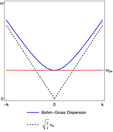
Bohm Gross
This dispersion function now accounts for how occupations in the plasma propagate.
\begin{equation}D\left(\vec{x},\vec{k},\omega\right)=\omega_{pe}+\frac{3}{2}\vec{k}\cdot\vec{k}v^{2}_{th}-\omega^{2}\equiv 0 \end{equation}
It has no resonances. Waves cannot propagate below \(\omega_{pe}\) and \(v_{g}\) can never exceed \(v_{th}\).
Ordinary Wave
This dispersion function represents a wave with a \(\vec{E}_{1}||\vec{B}_{0}\). That means the electric field occilates parallel to the magnetic field.
\begin{equation}D\left(\vec{x},\vec{k},\omega\right)=1-\frac{\omega^{2}_{pe}}{\omega^{2}}-\vec{n}_{\perp}\cdot\vec{n}_{\perp}\equiv 0 \end{equation}
This wave is cut off below \(\omega_{pe}\).

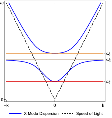
Extra Ordinary Wave
This dispersion function represents a wave with a \(\vec{E}_{1}\perp\vec{B}_{0}\). That means the electric field occilates perpendicular to the magnetic field.
\begin{equation}D\left(\vec{x},\vec{k},\omega\right)=1-\frac{\omega_{pe}^2}{\omega^{2}}\frac{\omega^{2}-\omega_{pe}^2}{\omega^{2}-\omega_{h}^2}-\vec{n}_{\perp}\cdot\vec{n}_{\perp}\equiv 0 \end{equation}
This mode has This wave has two branches. One branch is cannot not propagate below the \(\omega_{r}\) cutoff. The other branch cannot not propagate below the \(\omega_{l}\) cutoff. As the wave approaches the upper hybrid frequency, wave propagation stops as the wave number approaches \(\left|\vec{k}\right|\rightarrow\infty \).
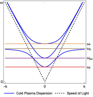
Cold Plasma
This dispersion function represents a wave in a cold plasma medium.
\begin{equation}D\left(\vec{x},\vec{k},\omega\right)=det\left(\vec{\epsilon}+\vec{n}\vec{n}-\vec{n}\cdot\vec{n}\vec{I}\right)\equiv 0 \end{equation}
The quantity \(\vec{\epsilon}\) is the dielectric tensor. Using Onsager symmetries, this tensor is defined as
\begin{equation}\vec{\epsilon}=\left(\begin{array}{ccc}\epsilon_{11}&\epsilon_{12}&0\\-\epsilon_{12}&\epsilon_{11}&0\\0&0&\epsilon_{33}\end{array}\right)\end{equation}
where
\begin{equation}\epsilon_{11}=1-\sum_{s}\frac{\frac{\omega^{2}_{p}}{\omega^{2}}}{1-\frac{\Omega^{2}_{c}}{\omega^{2}}}\end{equation}
\begin{equation}\epsilon_{12}=-i\sum_{s}\frac{\frac{\Omega_{c}}{\omega}\frac{\omega^{2}_{p}}{\omega^{2}}}{1-\frac{\Omega^{2}_{c}}{\omega^{2}}}\end{equation}
\begin{equation}\epsilon_{33}=1-\sum_{s}\frac{\omega^{2}_{p}}{\omega^{2}}\end{equation}
Note here we are including the plasma frequency for ions as well. This dispersion function is effectively a super position of the O-Mode and X-Mode dispersion functions and as such has the same cutoffs and resonances.
Developing new dispersion functions
This section is intended for code developers and outlines how to create new dispersion functions. New dispersion functions can be created from a subclass of dispersion::dispersion_function or any other existing dispersion_function class and overloading class methods. For convenience the dispersion::physics class contains several defined physical constants.
When a new dispersion function is subclassed from dispersion::dispersion_function an implementation must be provided for the pure virtual method dispersion::dispersion_function::D.
Supporting generalized coordinates
The dispersion::dispersion_interface assumes these are generalized coordinates. Developers must use the contravariant basis vector any time they compute the wave number vector.