Discription

Table of Contents

• Introduction
  • Graphs
    • Building Graphs
  • discription_workflows

A discription of the basic functions of the graph_framework.

Introduction

The basic functionality of this framework is to build expression graphs representing mathematical equations. Reduce those graphs to simpler forms. Transform those graph to take derivatives. Just-In-Time (JIT) compile them to available compute device kernels. Then run those kernels in workflow. The code is written in using C++23 features. To simplify embedding into legacy codes, there are additional language bindings for C and Fortran.

Graphs

Mathematical operations are defined as a tree of operations. A df method transforms the tree by applying the derivative chain rule to each node. A reduce method applies algebraic rules removing nodes from the graph.

The foundation of this framework is build around a tree data structure that enables the symbolic evaluation of mathematical expressions. The graph namespace contains classes which symbolically represent mathematical operations and symbols. Each node of the graph is defined as a class derived from a graph::leaf_node base class. The graph::leaf_node class defines method to graph::leaf_node::evaluate, graph::leaf_node::reduce, graph::leaf_node::df, graph::leaf_node::compile, and methods for introspection. A feature unique to this framework is the expression trees can be rendered to \(\LaTeX\) allowing a domain physicist to understand the results of reductions and transformations. This can also be used to identify future reduction opportunities.

An important distinction of this framework compared to other auto differentiation frameworks is there is no distinction between nodes representing operations and nodes representing values. Sub-classes of graph::leaf_node include nodes for constants, variables, arithmetic, basic math functions, and trigonometry functions. Other nodes encapsulate more complex expressions like piecewise constants which depend on the evaluation of an argument. These piecewise constants are used implement spline interpolation expressions.

Each node is constructed via factory methods. For common arithmetic operations, the framework overloads the +-*\/ operators to construct expression nodes. The factory method checks a node_cache to avoid building duplicate sub-graphs. Identification of duplicate graphs is performed by computing a hash of the sub-graph. This hash can be rapidly checked if the same hash already exists in a std::map container. If the sub-graph already exists, the existing graph is returned otherwise a new sub-graph is registered in the node_cache.

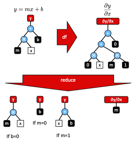
Each time an expression is built, the reduce method is called to simplify the graph. For instance, a graph consisting of constant added to a constant will be reduced to a single constant by calling the evaluate method. Sub-graph expressions are combined, factored out, or moved to enable better reductions on subsequent passes. As new ways of reducing the graph are implemented, current and existing code built using this framework benefit from improved speed. The figure above shows a visualization of the tree data structure for the equation of a line, the derivative, and the subsequent reductions.

Building Graphs

As an example building an expression of line \(y=mx+b\) accomplished by creating a graph::variable_node then applying operations on that node.

auto x = graph::variable<float> (10, "x");
auto y = 0.5*x + 0.1;

In this example, we have created a graph::variable_node with the symbol \(x\) containing 10 elements. Then built the expression tree for \(y\). Derivatives are taken using the graph::leaf_node::df method.

auto dydx = y->df(x);

Reductions are performed transparently as expressions are created so the expression for \(\frac{\partial y}{\partial x}=0.5\). As noted before, since this framework makes no distinction between the various parts of a graph, derivatives and also be taken with respect to sub-expressions.

auto dydmx = y->df(0.5*x);

In this case, the result will be \(\frac{\partial y}{\partial 0.5*x}=1.0\)

discription_workflows

A workflow::manager is responsible for compiling device kernels, and running them in order. One workflow::manager is created for each device or thread. The user is responsible for creating threads. Each kernel is generated through a workflow::work_item. A work item is defined by kernel graph::input_nodes, graph::output_nodes and graph::map_nodes. Map items are used to take the results of kernel and update an input buffer. Using our example of line equation, we can create a workflow to compute \(y\) and \(\frac{\partial y}{\partial x}\).

workflow::manager<T> work(0);
work.add_item({
    graph::variable_cast(x)
}, {
    y,
    dydx
}, {}, NULL, "example_kernel", 10);

Here we have defined a kernel called "example_kernel". It has one input \(x\), two outputs \(y\) and \(\frac{\partial y}{\partial x}\), and no maps. The NULL argument signifies there is no graph::random_state used. The last argument needs to match the number of elements in the inputs. Multiple work items can be created and will be executed in order of creation.

Once the work items are defined that can be JIT compiled to a backend device. The graph framework supports back ends for generic CPUs, Apple Metal GPUs, Nvidia Cuda GPUs, and initial HIP support of AMD GPUs. Each back end supplies relevant driver code to build the kernel source, compile the kernel, build device data buffers, and handle data synchronization between the device and host. All JIT operations are hidden behind a generic jit::context interface.

Each context, creates a specific kernel preamble and post-fix to build the correct syntax. Memory access is controlled by loading memory once in the beginning, and storing the results once at the end. Kernel source code is built by recursively traversing the output nodes and calling the graph::leaf_node::compile method of each graph::leaf_node. Each line of code is stored in a unique register variable assuming infinite registers. Duplicate code is eliminated by checking if a sub-graph has already been traversed. Once the kernel source code is built, the kernel library is compiled, and a kernel dispatch function is created using a C++ lambda function. The resulting workflow can be called multiple times.

work.compile();
for (size_t i = 0; i < 100; i++) {
    work.run();
}
work.wait();

While this API is more explicit compared to the capabilities of JAX, PyTorch, TensorFlow, and MLX, it doesn't result in unexpected situations where graphs are being rebuilt and the user can trust when evaluation is finished. Additionally device buffers are only created for kernel inputs and outputs allowing the user to explicitly control memory usage.