Introduction

This page documents the types and formatting of the equilibrium models. xrays currently supports two equilibrium models.

EFIT Are 2D axisymetric equilibria relevant to tokamak devices.
VMEC Are 3D nested flux surface equilibria relevant for stellarator devices.

This documentation assumes the user has some familiarity with EFIT or VMEC and focuses instead how quanties from these are formatted.

Spline Formatting

The equilibrium models used in this section make use of Cubic and Bicubic splines.

Cubic Splines

Cubic splines are 1D interpolation functions consisting of 4 coeffient arrays. They take the form of

\begin{equation}y\left(x\right)=C_{0} + C_{1}x + C_{2}x^2 + C_{3}x^2\end{equation}

where \(x\) is a normalized radial index. Cubic splines coefficients can be calculated using Linear Solvers However, to avoid needing account for index offsets, index offsets are pre computed into the spline coefficents.

\begin{equation}C'^{i}_{0}=C^{i}_{0} - C^{i}_{1}i + C^{i}_{2}i^2 - C^{i}_{3}i^3\end{equation}

\begin{equation}C'^{i}_{1}=C^{i}_{1} -2C^{i}_{2}i + 3C^{i}_{3}i^2\end{equation}

\begin{equation}C'^{i}_{2}=C^{i}_{2} - 3C^{i}_{3}i\end{equation}

\begin{equation}C'^{i}_{3}=C^{i}_{3}\end{equation}

Where \(i\) is the index of the coeffient array. This allows to normalize the spline argument \(x\) so that it can both index the array and evaluate the spline.

\begin{equation}x = \frac{x_{real} - x_{min}}{dx}\end{equation}

Rounding down the value of \(x\) gives the correct coefficient index.

Bicubic Splines

Bicubic Splines are computed in a simular way instead they consist of a total of 16 coeffients. These represent 4 spline functions in one dimension which interpolate 4 coeffient values for the other dimension. Like the 1D splines, 2D spline coeffients are normalized so the spline arguments can be used as normalized indices.

\begin{equation}C'^{ij}_{00}=C^{ij}_{00}-C^{ij}_{01}j+C^{ij}_{02}j^{2}-C^{ij}_{03}j^{3}-C^{ij}_{10}i+C^{ij}_{11}ij-C^{ij}_{12}ij^{2}+C^{ij}_{13}ij^{3}+C^{ij}_{20}i^{2}-C^{ij}_{21}i^{2}j+C^{ij}_{22}i^{2}j^{2}-C^{ij}_{23}i^{2}j^{3}-C^{ij}_{30}i^{3}+C^{ij}_{31}i^{3}j-C^{ij}_{32}i^{3}j^{2}+C^{ij}_{33}i^{3}j^{3}j\end{equation}

\begin{equation}C'^{ij}_{01}=C^{ij}_{01}-2C^{ij}_{02}j+3C^{ij}_{03}j^{2}-C^{ij}_{11}i+2C^{ij}_{12}ij-3C^{ij}_{13}ij^{2}+C^{ij}_{21}i^{2}-2C^{ij}_{22}i^{2}j+3C^{ij}_{23}i^{2}j^{2}-C^{ij}_{31}i^{3}+2C^{ij}_{32}i^{3}j-3C^{ij}_{33}i^{3}j^{2}\end{equation}

\begin{equation}C'^{ij}_{02}=C^{ij}_{02}-3C^{ij}_{03}j-C^{ij}_{12}i+3C^{ij}_{13}ij+C^{22}i^{2}-3C^{ij}_{23}i^{2}j-C^{ij}_{32}i^{3}+3C^{ij}i^{3}j \end{equation}

\begin{equation}C'^{ij}_{03}=C^{ij}_{03}-C^{ij}_{13}i+C^{ij}_{23}i^{2}-C^{ij}_{33}i^{3}\end{equation}

\begin{equation}C'^{ij}_{10}=C^{ij}_{10}-2C^{ij}_{11}j+C^{ij}_{12}j^{2}-C^{ij}_{13}j^{3}-2C^{ij}_{20}i+2C^{ij}_{21}ij-2C^{ij}_{22}ij^{2}+2C^{ij}_{23}ij^{3}j+3C^{ij}_{30}i^{2}-3C^{ij}_{31}i^{2}j+3C^{ij}_{32}i^{2}j^{2}-3C^{ij}_{33}i^{2}j^{3}\end{equation}

\begin{equation}C'^{ij}_{11}=C^{ij}_{11}-2C^{ij}_{12}j+3C^{ij}_{13}j^{2}-2C^{ij}_{21}i+4C^{ij}_{22}ij-6C^{ij}_{23}ij^{2}+3C^{ij}_{31}i^{2}-6C^{ij}_{32}i^{2}j+9C^{ij}_{33}i^{2}j^{2}\end{equation}

\begin{equation}C'^{ij}_{12}=C^{ij}_{12}-C^{ij}_{13}j-2C^{ij}_{22}i+6C^{ij}_{23}ij+3C^{ij}_{32}j-9C^{ij}_{33}i^{2}j \end{equation}

\begin{equation}C'^{ij}_{13}=C^{ij}_{13}-2C^{ij}_{23}i+3C^{ij}_{33}i^{2}\end{equation}

\begin{equation}C'^{ij}_{20}=C^{ij}_{20}-C^{ij}_{21}j+C^{ij}_{22}ij^{2}-C^{ij}_{23}j^{3}-3C^{30}i+3C^{ij}_{31}ij-3C^{ij}_{32}ij^{2}+3C^{ij}_{33}ij^{3}\end{equation}

\begin{equation}C'^{ij}_{21}=C^{ij}_{21}-2C^{ij}_{22}j+3C^{ij}_{23}j^{2}-3C^{ij}_{31}i+6C^{32}ij-9C^{ij}_{33}ij^{2}\end{equation}

\begin{equation}C'^{ij}_{22}=C^{ij}_{22}-3C^{ij}_{23}j-3C^{ij}_{32}i+9C^{ij}_{33}ij \end{equation}

\begin{equation}C'^{ij}_{23}=C^{ij}_{23}-3C^{ij}_{33}i \end{equation}

\begin{equation}C'^{ij}_{30}=C^{ij}_{30}-C^{ij}_{31}j+C^{ij}_{32}j^{2}-C^{ij}_{33}j^{3}\end{equation}

\begin{equation}C'^{ij}_{31}=C^{ij}_{31}-2C^{ij}_{32}j+3C^{ij}_{32}j^{2}\end{equation}

\begin{equation}C'^{ij}_{32}=C^{ij}_{32}-3C^{ij}_{33}j \end{equation}

\begin{equation}C'^{ij}_{33}=C^{ij}_{33} \end{equation}

Bicubic splines are computed by

\begin{equation}f\left(x,y\right)=\left(\begin{array}{cccc}1 & x & x^{2} & x^{3}\end{array}\right)\cdot\left(\left(\begin{array}{cccc}C_{00}&C_{01}&C_{02}&C_{03}\\C_{10}&C_{11}&C_{12}&C_{13}\\C_{20}&C_{21}&C_{22}&C_{23}\\C_{30}&C_{31}&C_{32}&C_{33}\end{array}\right)\cdot\left(\begin{array}{c}1\\y\\y^{2}\\y^{3}\end{array}\right)\right)\end{equation}

Like the 1D splines \(x\) and \(y\) are normalized.

\begin{equation}x = \frac{x_{real} - x_{min}}{dx}\end{equation}

\begin{equation}y = \frac{y_{real} - y_{min}}{dy}\end{equation}

EFIT

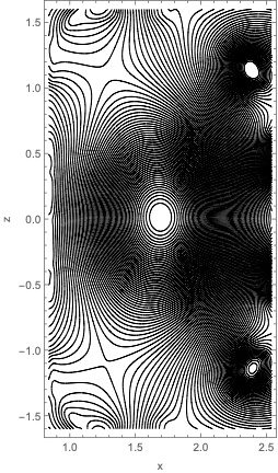
Cross section of poloidal flux surfaces.

EFIT is an equilibium that comes from a solution of the Grad–Shafranov equation. The solution gives us a map of the poloidal flux \(\psi\) on 2D grid and a 1D flux function \(f_{pol}\). 1D profiles of electrion density \(n_{e}\left(\psi\right)\), electron temperature \(t_{e}\left(\psi\right)\), and pressure \(p\left(\psi\right)\) are mapped as functions of the normalized flux.

EFIT file format

Quantities are loaded into the ray tracer via a netcdf file. EFIT NetCDF files must contain the following quantities. Spline quanities have a common format of name_ci or name_cij.

Efit netcdf file quantities
Dimensions
Name		Discription
`numr`		Size of radial grid.
`numz`		Size of vertical grid.
`numpsi`		Size of arrays for \(\psi\) mapped quantities.
Scalar Qantities
`dpsi`		Step size of the \(\psi\) grid.
`dr`		Step size of the radial grid.
`dz`		Step size of the vertial grid.
`ne_scale`		Scale of the \(n_{e}\) profile.
`pres_scale`		Scale of the pressure profile.
`psibry`		Value of \(\psi\) at the boundary.
`psimin`		Minimum \(\psi\) value.
`rmin`		Minimum radial value.
`te_scale`		Scale of the electron temperature profile.
`zmin`		Minimum vertial value.
1D Qantities
Name	Size	Discription
`fpol_ci`	`numpsi`	Flux function profile coefficents
`ne_ci`	`numpsi`	\(n_{e}\) profile coefficents.
`pressure_ci`	`numpsi`	Pressure profile coefficents.
`te_ci`	`numpsi`	\(t_{e}\) profile coefficents.
2D Qantities
Name	Size	Discription
`psi_cij`	`(numr,numz)`	\(\psi\left(r,z\right)\) coefficents.

VMEC

Cross section of 3D flux surfaces.

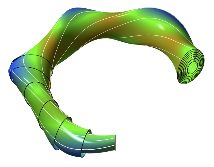
VMEC is an equilibium that comes from minimizing mhd energy. The solution gives us set of Fourier coefficents on a discrete radial grid. 1D profiles of electrion density \(n_{e}\left(\psi\right)\), electron temperature \(t_{e}\left(\psi\right)\), and pressure \(p\left(\psi\right)\) are mapped as functions of the normalized flux.

VMEC file format

Quantities are loaded into the ray tracer via a netcdf file. VMEC NetCDF files must contain the following quantities. Spline quanities have a common format of name_ci. All radial quantities are splined accross the magnetic axis to the opposite end. That is quantities extend from \(-s\rightarrow s \). Splines of fourier coeffients are one dimensional splines stored in a 2D array. Radial quantities are stored as a full or half grid value.

VMEC netcdf file quantities
Dimensions
Name		Discription
`numsf`		Size of full radial grid.
`numsh`		Size of half radial grid.
`nummn`		Number of Fourier modes.
Scalar Qantities
`dphi`		Step size of toroidal flux.
`ds`		Step size of normalized toroidal flux.
`signj`		Sign of the Jacobian.
`sminf`		Minimum \(s \) on the full grid.
`sminh`		Minimum \(s \) on the half grid.
1D Qantities
Name	Size	Discription
`chi_ci`	`numsf`	Poloidal flux profile.
`xm`	`nummn`	Poloidal modes.
`xn`	`nummn`	Toroidal modes.
2D Qantities
Name	Size	Discription
`lmns_ci`	`(numsh,nummn)`	\(\lambda \) fourier coefficents.
`rmnc_ci`	`(numsf,nummn)`	\(r \) fourier coefficents.
`zmns_ci`	`(numsf,nummn)`	\(z \) fourier coefficents.

Developing new equilibrium models

This section is intended for code developers and outlines how to create new equilibrium models. All equilibrium model use the same equilibrium::generic interface. New equilibrium models can be created from a subclass of equilibrium::generic or any other existing equilibrium class and overloading class methods.

template<jit::float_scalar T, bool SAFE_MATH=false>
class new_equilibrium final : public generic<T, SAFE_MATH> {
   ...
};

When a new equilibrium is subclassed from equilibrium::generic implimentations must be provided for the following pure virtual methods.

Note: equilibrium::generic::get_characteristic_field is only used by the normalized boris method for particle pushing. For most cases this can simply return 1.

For the remaining methods, or any other methods one wishes to override, the arguments provide expressions for the input position of the ray. The methods return are expressions for the quantity at hand.

Noncartesian Coordinates

While these methods take an \(x,y,z \) as the argument names, there is no reason these need to be assumed to be cartesian coordinates. For instance the VMEC treats \(x,y,z\rightarrow s,u,v \) as flux coordinates. In flux coordinate the coordinate system is no longer normalized nor orthogonal. So that other parts of the code can treat \(\vec{k}\) correctly there are methods to return the covariant basis vectors \(\vec{e}_{s},\vec{e}_{u},\vec{e}_{v}\).

By default, equilibrium::generic return basis vectors for a cartesian system \(\vec{e}_{1}=\hat{x},\vec{e}_{2}=\hat{y},\vec{e}_{3}=\hat{z}\).

Table of Contents