Introduction

This page documents general concepts of the graph_framework.

Definitions

Glossery of terms
Concept	Definition
node	A leaf or branch on the graph tree.
graph	A data stucture connecting nodes.
reduce	A transformation of the graph to remove leaf_nodes.
auto differentiation	A transformation of the graph build derivatives.
compiler	A tool for translating from one language to another.
JIT	Just-in-time compile.
kernel	A code function that runs on a batch of data.
pre_item	A kernel to run before running the main kernels.
work_iten	A instance of kernel.
converge_item	A kernel that is run until a convergence test is met.
workflow	A series of work items.
backend	The device the kernel is run on.
recursion	See definition of recursion.
safe math	Run time checks to avoid off normal conditions.
API	Application programming interface.
Host	The place where kernels are launched from.
Device	The side where kernels are run.

Graph

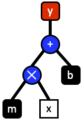
The graph_framework operates by building a tree structure of math operations. For an example of building expression structures see the basic expressions tutroial. In tree form it is easy to traverse nodes in the graph. Take the example of equation of a line.

\begin{equation}y=mx + b\end{equation}

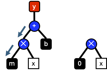
This equation consists of five nodes. The ends of the tree are clasified as either variables \(x\) or constants \(m,b\). These nodes are connected by nodes for multiply and addition operations. The output \(y\) represents the entire graph of operations.

The graph stucture for y = mx + b.

Evaluation of graphs start from the top most node in this case the \(+\) operation. Evaluation of a node is not performed until all subnodes are evaluated starting with the left operand. Evaluation starts by recursively evaluating the left operands until the last node is reached \(m\).

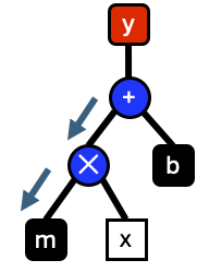
Once \(m\) the result is returned to the \(+\) then the right operand is evaluated.

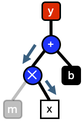
Evaluation is repeated until every node in the graph is evaluated.

Auto Differentiation

From the previous section, it was shown how graphs can be evaluated. This same evaluation can be applied to build graphs of a function derivative. For an example of taking derivatives see the auto differentiation tutroial. Lets say that we want to take the derivative of \(\frac{\partial y}{\partial x}\). This is achieved by evaluating the until bottom left most node is reached. Then a new graph is build starting with \(\frac{\partial m}{\partial x}=0\). Applying the first half of the chain rule we build a new graph for \(0x\)

Then we take the derivative of the right operand and apply the second half of the chain rule to build a new graph for \(0x=0\).

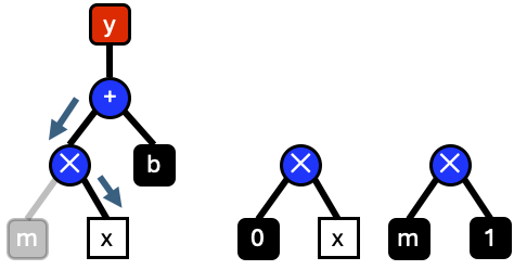
Evaluation is repeated recursively until the full graph has been evaluated.

Reduction

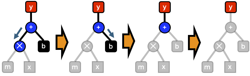
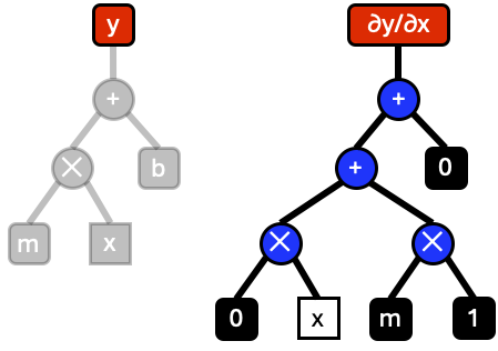
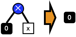
The final expression for \(\frac{\partial y}{\partial x}\) contains many unnecessary nodes in the graph. Instead of building full graphs, we can simplify and eleminate nodes as we build them. For instance, when the expression \(0x\) this created can be immediately reduce it to a single node.

Applying all possible reductions reduces the final expression to \(\frac{\partial y}{\partial x}=m\).

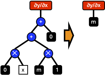
By reducing graphs as they are build, we can eliminate nodes one by one.

Compile

Once graph expressions are built, they can be compiled to a compute kernel. For an example of compiling expression trees into kernels see the workflow tutroial. Using the same recursive evaluation, we can visit each node of a graph and and create a line of kernel source code. There are three important parts for creating kernels, inputs, outputs, and maps. These three concepts define buffers on the compute device and how they are changed. Compute kernels can be genereted from multiple outputs and maps.

Inputs

Inputs are the variable nodes that define the graph inputs. In the line example \(\frac{\partial y}{\partial x}\), the input variable would be the node for \(x\). Some graphs have no inputs. The graph for \(\frac{\partial y}{\partial x}=m\) has eliminated all the variable nodes in the graph.

Outputs

Outputs are the ends of the nodes. These are the values we want to compute. Any node of a graph can be a potential output. For each output a device buffer is generated to store the results of the evalutaion. For nodes that are not used as outputs, no buffers need to be created since those results are never stored.

Maps

Maps enable the results of an output node to be stored in an input node. This is use for a wide varity of steps. For instance take a gradient decent step.

\begin{equation}y = y + \frac{\partial f}{\partial x}\end{equation}

In this case the output of the expression \(y + \frac{\partial f}{\partial x}\) can be mapped to update \(y\).

Workflows

Sequences of kernels are evaluated in workflow. A workflow is defined from workitems which wrap a kernel call.

Safe Math

There are some conditions where mathematically, a graph should evaluate to a normal number. However, when evaluted suing floating point precison, can lead to Inf or NaN. An example of this the \(\exp\left(x\right)\) function. For large argument values, \(\exp\left(x\right)\) overflows the maximum floating point precision and returns Inf. \(\frac{1}{\exp\left(x\right)}\) should evaluate zero however, in floating point this becomes a NaN. Safe math avoids problems like this by checking for large argument values. But since these run time checks slow down kernel evaluation, most of the time safe math should be avoided.

Table of Contents