Table of Contents
Examples of physics problems created with the graph_framework.
Introduction
There are many problems in fusion energy where the same equation needs to be applied to a large ensemble. This paper will highlight two examples using the graph framework. The first is an RF ray tracing problem to determine plasma heating. The second example is for particle pushing.
RF Ray tracing
Geometric optics is a set of asymptotic approximation methods to solve wave equations. The physics of the particular wave determines an algebraic relation between \(\omega\) and \(\vec{k}\) called a dispersion relation, \(D\left(\omega,\vec{k}\right)=0\). Since the parameter \(t\) does not appear explicitly in the dispersion relation, the function \(\omega\left(\vec{k}\left(t\right),\vec{x}\left(t\right)\right)\) is constant along the ray trajectory
\begin{equation}\frac{\partial\omega}{\partial t}=\frac{\partial\omega}{\partial\vec{x}}\cdot\frac{\partial\vec{x}}{\partial t}+\frac{\partial\omega}{\partial\vec{k}}\cdot\frac{\partial\vec{k}}{\partial t}\equiv 0\end{equation}
by virtue of the ray equations. Since the dispersion relation is satisfied all along the ray trajectory, the derivatives needed for the ray equations can be obtained by implicit differentiation
\begin{equation}\frac{\partial D}{\partial\vec{x}}=\frac{\partial D}{\partial\omega}\frac{\partial\omega}{\partial\vec{x}}\Rightarrow\frac{\partial\omega}{\partial\vec{x}}=-\frac{\frac{\partial D}{\partial\vec{x}}}{\frac{\partial D}{\partial\omega}}\end{equation}
\begin{equation}\frac{\partial D}{\partial\vec{k}}=\frac{\partial D}{\partial\omega}\frac{\partial\omega}{\partial\vec{k}}\Rightarrow\frac{\partial\omega}{\partial\vec{k}}=-\frac{\frac{\partial D}{\partial\vec{k}}}{\frac{\partial D}{\partial\omega}}\end{equation}
These equations are integrated to trace the ray.
A ray tracing problem is build by implementing expressions for the plasma equilibrium. From the plasma equilibrium a dispersion relation is constructed. Equations of motion are defined using the auto differentiation. Expressions for ray update are built for in integrator. These expressions are JIT compiled into a single kernel call with inputs for \(\vec{x}\), \(\vec{k}\), \(t\), and \(\omega\) with outputs for the dispersion residual, and step updates for \(\vec{x}\), \(\vec{k}\) and \(t\).
Correctness
Here we illustrate the correctness of the code by examining waves described by relatively simple dispersion relations in plane stratified plasmas, that is plasma with spatial variation only in the \(x\) direction. In a spatially varying medium, at a given frequency, there may be regions in which the solution of the dispersion relation, \(\vec{k}\), is real, and the wave propagates. In other regions \(\vec{k}\) is imaginary and the wave does not propagate, referred to as evanescent. The boundary between a region of propagation and evanescence is a surface called a cut-off. It is also possible that surfaces occur where \(\vec{k}\) diverges to infinity, in which case the phase velocity component normal to the surface goes to zero. These are called resonances. Typically, the wave is reflected at a cut-off and is absorbed or converted to a different type of wave at a resonance. These critical surfaces, therefore, demark important changes in wave behavior, and the behavior of rays in their vicinity is an indication of the correctness of the solution.
For plasmas, the spatial dependence of the dispersion relation comes through variation of the plasma equilibrium quantities. These include the vector magnetic field, \(\vec{B}\left(x\right)\), the density of each plasma particle species, \(n_{s}\left(x\right)\), and the temperature of each particle species, \(T_{s}\left(x\right)\), where \(s\) indicates a particular species. For the cases presented here a linear gradient along the \(x\) direction is taken for either the particle density or magnetic field strength.
\begin{equation}f\left(x\right)=0.1x+1\end{equation}
Unless otherwise noted, the following table lists values for the plasma conditions.
| Symbol | Value |
|---|---|
| \(m_{i}\) | \(3.344\times10^{-27}\) kg |
| \(n_{e0}\) | \(1\times10^{19}\) m \(^{-3}\) |
| \(n_{i0}\) | \(n_{e0}\) |
| \(T_{e}\) | \(1\) keV |
| \(T_{i}\) | \(T_{e}\) |
| \(\vec{B}\) | \(1\) T \(\hat{z}\) |
The examples presented employ the Cold Plasma approximation. This means that the particle thermal speeds are much less than the wave phase velocity and the magnetic field is sufficiently strong that the particle gyro-radius is much less than the wavelength. The cold-plasma approximation greatly simplifies the dispersion relation and is actually valid for a wide range of wave propagation situations of fusion interest. A further approximation is made that the wave frequency is so high that only the electrons respond to the wave fields and the much heavier ions do not contribute to the wave-induced plasma current.
Initial conditions for the wave solution are obtained by choosing fixed values for \(\omega\), \(\vec{x}\), \(k_{y}\), and \(k_{z}\). The remaining value \(k_{x}\) is solved for using a Newton method to a tolerance of \(\left|D\left(\vec{k},\omega\right)\right|<10^{-15}\). Since the dispersion functions are multi-valued, an initial guess for \(k_{x}\) selects among the possible roots.
To mitigate the effects of floating point round-off errors, terms in the dispersion relation are combined to reduce the orders of magnitude for quantities. In plasmas, frequencies and waves typically trend in the \(100\) GHz range. Folding the speed of light into the frequency, \(\omega'=\frac{\omega}{c}\), results in quantities of \(\omega'\) on the order of \(1000\). The consequence is that this modified frequency \(\omega'\) has units of m \(^{-1}\). The phase, \(v_{p}=\frac{\omega}{k}\), and group, \(v_{g}=\frac{\partial\omega}{\partial k}\), velocities are unit less. As a consequence, time now contains a speed of light term \(t'=tc\) with units of m. This slows time from values on the order of \(1\times10^{-7}\) to \(1\). Under this scheme, quantities of interest for ray tracing, position, \(\vec{x}\), and wave number, \(\vec{k}\), retain their normal units. The Normalization table, summarizes the changes resulting from these modified units. The following results are converted back to real units unless otherwise indicated.
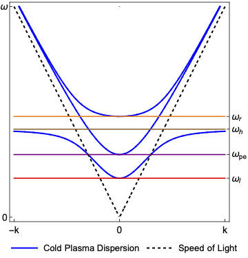
The figure above shows the dispersion relation for a uniform magnetic field and density gradient. This dispersion is a superposition of the Ordinary Wave and Extra Ordinary Wave dispersion relations. For a given frequency, one branch can cross cutoffs and resonances, the other cannot.
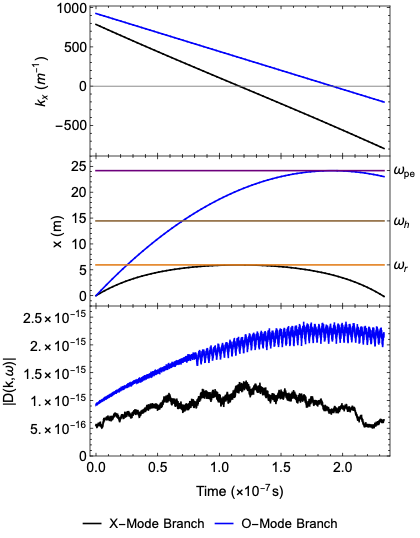
The figure above shows the wave trajectories for two waves above \(\omega_{r}\). The O-Mode branch can pass \(\omega_{r}\) while the X-Mode branch is reflected.

The figure above shows the wave trajectories for two waves between \(\omega_{h}\) and \(\omega_{l}\). The X-Mode branch can pass \(\omega_{pe}\) cutoff while the O-Mode branch is reflected. The X-Mode branch is absorbed in the upper hybrid resonance, \(\omega_{h}\), while the O-Mode branch can pass through it.
Correctness
Genray is an RF-Ray tracing code written in Fortran which operates in a cylindrical geometry. Toroidal equilibria can be imported using the EFIT EQDSK format. Derivative information must either be explicitly defined or used a numerical differentiation. Since Genray does not trace within the vacuum region care was taken to ensure the two codes started from the same initial conditions. A single ray was traced in Genray then initial position and wave number was used to initialize the Graph framework ray tracer. Additionally the plasma profiles from Genray were matched with expression in the graph framework.
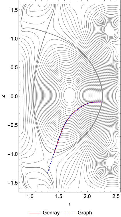
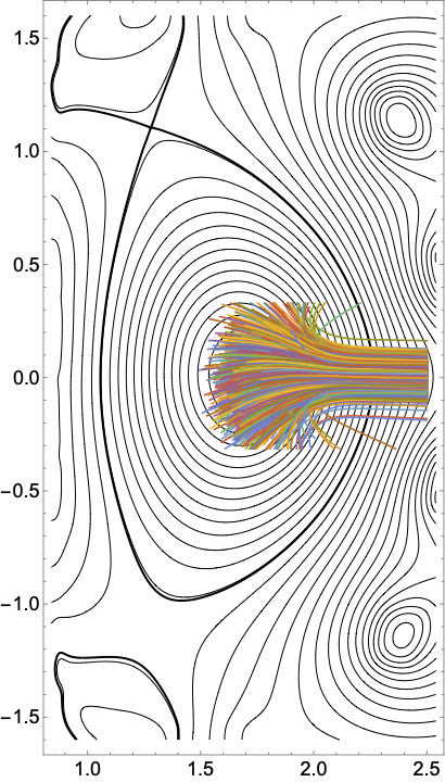
The figure above shows the trajectory of rays in the a tokamak cross-section. Both codes show a nearly identical trajectory with only a slight deviation towards the end of ray.
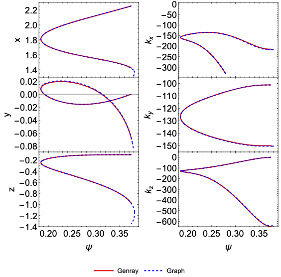
The figure above shows the comparison of wave position \(\vec{x}\) and wave number \(\vec{k}\). Since the two codes use different time steps, these are plotted with respect to the flux label \(\psi\). Both codes show nearly identical results with only a small deviation towards the end of the trace.
Particle Pushing
In order to achieve good statistics for the evolution of particle distributions, it's necessary to push large numbers of particles. Exploiting GPU resources is necessary to achieve the large number of particles at reasonable run times to enable self consistent fields. An example is the runaway electron problem.
During a disruption in a tokamak, electric fields can drive electron beams up to relativistic speeds. These high energy particles can lose confinement and damage first wall components. The Boris leap-frog algorithm can integrate particles while conserving energy and momentum. The algorithm updates particle position \(\vec{x}\), momentum \(\vec{u}\), and relativistic \(\gamma\).
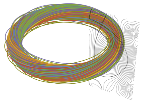
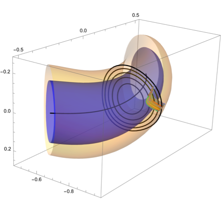
The Figure above shows \(100\) out of \(10^{5}\) particles trajectories in a realistic tokamak geometry.