Add low fidelity engineering modeling
In this section, a few simplified engineering models are added to the example4
Evaulation
Command line
evaluate.py --input=evaluate.json --output=evaluate.dat --nsample=100000 --quiet
evaluate.json
{
  "scan": {
    "d_blanket" : {"type": "range", "ymin":0.2, "ymax":0.4},
    "d_tf"      : {"type": "range", "ymin":0.4, "ymax":1.2},
    "d_cs"      : {"type": "range", "ymin":0.2, "ymax":0.6},
    "f_wp"      : {"type": "range", "ymin":0.5, "ymax":0.8},
    "f_r_tf_out": {"type": "range", "ymin":2.5, "ymax":4.5}
  },

  "const": {
    "aratio"      : 3.0,
    "a"           : 1.3333,
    "kappa"       : 2.0,
    "delta"       : 0.6,
    "bt"          : 7.0,
    "ip"          : 8.1,

    "pinj"        : 38.0,
    "fgw_ped"     : 1.0,
    "nepeak"      : 1.9,
    "h98"         : 1.4,

    "eta_cd"      : 0.25,
    "eta_th"      : 0.33,

    "d_sol"       : 0.1,
    "d_str"       : 0.1,
    "gap_vv"      : 0.05,
    "d_vv"        : 0.15,
    "gap_shield"  : 0.05,
    "d_shield"    : 0.225,
    "gap_tf"      : 0.083,
    "gap_cs"      : 0.08,

    "t_helium"    : 4.5,
    "strain_sc"   : -0.005,
    "f_sc_copper" : 0.69,
    "f_sc_helium" : 0.46,
    "f_sc_conductor": 0.28
  },

  "model": {
    "r"         : ["expr", "a * aratio"                 ],
    "betan_ped" : ["base", {}   ],
    "te_ped"    : ["base", {"dependency":"betan_ped"}   ],
    "ti_ped"    : ["expr", "te_ped"                     ],
    "ngw"       : ["base", {}                           ],
    "ne_ped"    : ["expr", "fgw_ped * ngw"              ],
    "ne_axis"   : ["expr", "nepeak * ne_ped"            ],
    "betan"     : ["file", "fitout.json" ],
    "pfus"      : ["file", "fitout.json" ],
    "fbs"       : ["file", "fitout.json" ],
    "pnet"      : ["base", {}],

    "d_wp"      : ["expr", "f_wp * d_tf"],
    "r_tf"      : ["expr", "r - ( a + d_sol + d_blanket + d_str + gap_vv + gap_shield + d_shield + gap_tf + d_tf )"],
    "r_cs"      : ["expr", "r_tf - ( gap_cs + d_cs )"],
    "r_tf_out"  : ["expr", "r + f_r_tf_out * a"],

    "bmax"      : ["base", {}],
    "itf"       : ["base", {}],
    "jtf"       : ["base", {}],
    "tf_stress_axial" : ["base", {}],
    "tf_stress_hoop"  : ["base", {}],
    "tf_stress" : ["expr", "tf_stress_axial + tf_stress_hoop"],
    "jsc_crit"  : ["base", {}],
    "jtf_crit"  : ["expr", "jsc_crit * f_sc_copper * f_sc_helium * f_sc_conductor" ],
    "f_jtf_crit": ["expr", "jtf / jtf_crit"]
  }

}
For the illustration purpose, one of the simplified radial build models is employed, which is mainly defined by the inboard thicknesses for a set of the tokamak structures including blanket (d_blanket), structure ring (d_str), vacuum vessel (d_vv), thermal shield (d_shield), TF coil (d_tf), and central solenoid (d_cs), along with the gaps between the structures (gap_vv, gap_shield, gap_tf, gap_cs). See the parametric geometry representation of tokamak and the definition of TokDesinger variables
For the CAT-like reference case (aratio = 3, pinj = 38 MW, fgw_ped = 1, h98 = 1.4), this example evaluates:
- TF coil stress (
tf_stress) = sum of the hoop (tf_stress_hoop) and axial (tf_stress_axial) stresses - TF coil current density in the winding pack (
jtf) to produce the target magnetic field (bt= 7 T at the plasma geometry centerr= 4 m) - TF coil current density limit in the winding pack (
jtf_crit) imposed by the critical superconductor coil current density (jsc_crit).
for a range of the radial build dimensions, in particular to decide a feasible thickness range of TF coil (d_tf) and blanket (d_blanket).
Filtering
The constraints used in this example are:
tf_stress< 500 MPajtf<jtf_critr_cs> 0.2 m
, where r_cs is the inner radius of central solenoid.
Command line
filter.py --input=filter.json --dbfile=evaluate.dat --output=filter.dat
filter.json
{
"filter": {
  "tf_stress" : ["max", 500.0],
  "f_jtf_crit"  : ["max", 1.0],
  "r_cs" : ["min", 0.2]
}
}
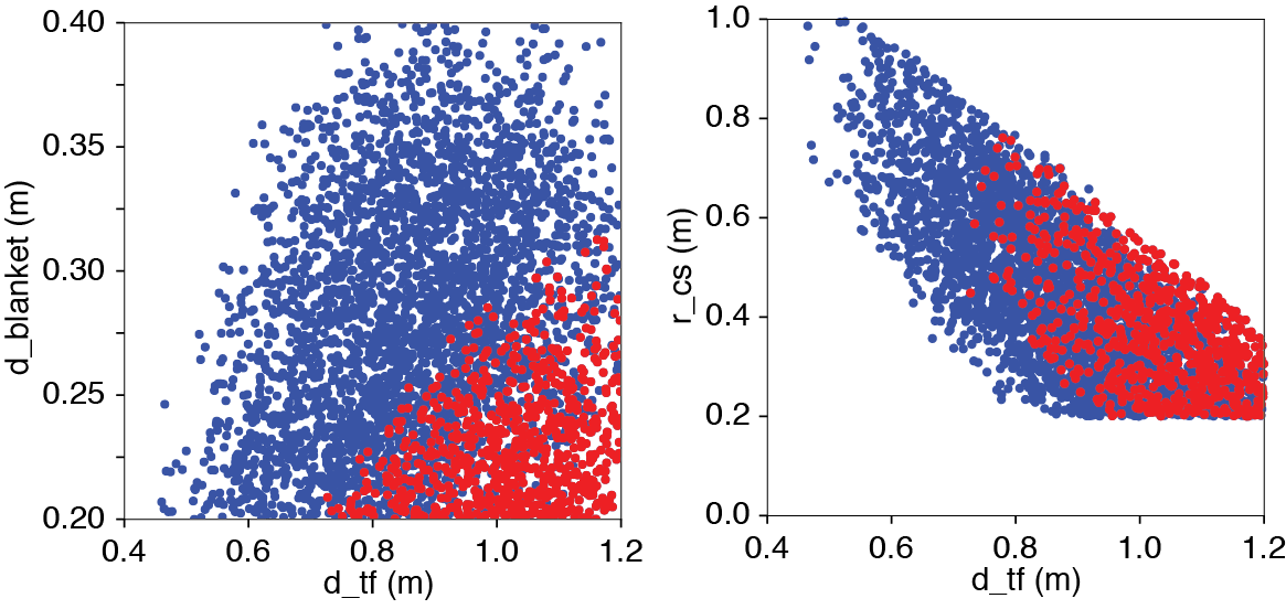
The blue + red points satisfy the radial build (r_cs > 0.2) and the TF coil stress constraint (tf_stress < 500 MPa). The red points satisfy additional superconductor current limit (jtf < jtf_crit).