Evaluate and apply filitering
This step illustrates how to evaluates the reactor performace parameters using the reduced system model developed in the previous section and filter for the desired reactor performance.
Evaulation
This example uses the reduced model file fitout.json from the previous section for the fbs, pfus, and betan. The net electricity pnet model is a TokDiesigner base model.
Command line
evaluate.py --input=evaluate.json --output=evaluate.dat --nsample=100000
The evaluate.py generates a database file evaluate.dat in a multi-dimensional parameter space of aratio, pinj, fgw_ped, nepeak, and h98 for the --nsample random data points (100,000 points).
Note
In this example, the range of the scan variables is same to the random sampling range for IPS-FASTRAN (Scan with Random Sampling). The extrapolation outside of the model data generation range is often employed with the Log-linear model but not likely accurate for the Neural Network model.
evaluaion.json
 {

 "scan": {
   "aratio"    : {"type": "range", "ymin":2.5, "ymax":3.5},
   "pinj"      : {"type": "range", "ymin":20.0, "ymax":50.0},
   "fgw_ped"   : {"type": "range", "ymin":0.7, "ymax":1.0},
   "nepeak"    : {"type": "range", "ymin":1.5, "ymax":2.0},
   "h98"       : {"type": "range", "ymin":0.9, "ymax":1.5}
 },

 "const": {
   "a"       : 1.3333,
   "kappa"   : 2.0,
   "delta"   : 0.6,
   "bt"      : 4.0,
   "ip"      : 8.1,
   "eta_cd"  : 0.25,
   "eta_th"  : 0.33
 },

"model": {
   "r"          : ["expr", "a * aratio"                 ],
   "betan_ped"  : ["base", {}   ],
   "te_ped"     : ["base", {"dependency":"betan_ped"}   ],
   "ti_ped"     : ["expr", "te_ped"                     ],
   "ngw"        : ["base", {}                           ],
   "ne_ped"     : ["expr", "fgw_ped * ngw"              ],
   "ne_axis"    : ["expr", "nepeak * ne_ped"            ],
   "betan"      : ["file", "fitout.json" ],
   "pfus"       : ["file", "fitout.json" ],
   "fbs"        : ["file", "fitout.json" ],
   "pnet"       : ["base", {}]
 }

 }
The content and format of the input file evaluate.json is identical to the sample.json except without the io section (see Scan with Random Sampling). Note that the model section for the betan, pfus, and fbs points to the reduced model file fitout.json.
Filtering
The process is same to the Direct Filtering but with the database file evaluate.dat generated by the reduced system model.
Command line
filter.py --input=filter.json --dbfile=evaluate.dat --output=filter.dat
filter.json
{
"filter": {
  "fbs"  : ["min", 0.8],
  "fbs"  : ["max", 1.0],
  "pnet" : ["min", 50.0]
}
}
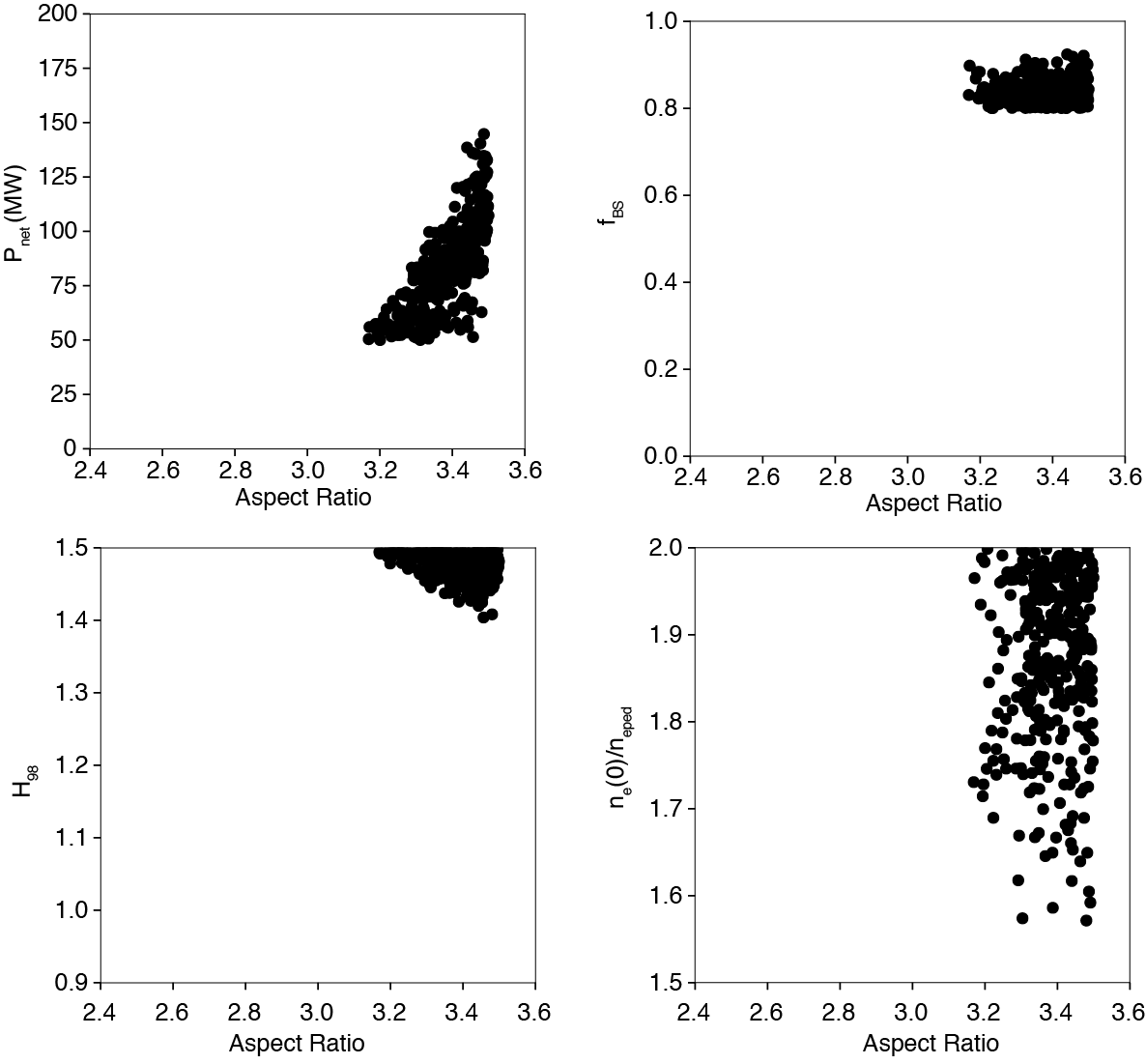
This is an example for the bootstrap current 0.8 <= fbs <= 1.0 and the net electricity pnet >= 50 MW. The output database file filter.dat contains the filtered points satisfying these constraints.
The indentified aratio range is aratio > 3.1 for 0.8 <= fbs <= 1.0 and pnet >= 50 MW, The results indicate that very high confinement h98 > 1.4 is required, but not necessarily high density peaking.
Warning
Many parameters in the scan in this example such as the toroidal field, current, minor radius etc are constant. The results should not read like higher aratio is better.