Generate reduced model

This step illustrates how to generate a Reduced System Model (RSM) from the random sampling scan in the previous section. The RSM is a parameterization of the global tokamak variable such as the normalized plasma pressure betaN, bootstrap current fraction fBS, toroidal field hoop stress stress_hoop etc as a function of the Tokamak design and operation parameters. TokDeisigner supports a range of Machine Learning techniques including Log-linear (LL) regression, Gaussian Process (GP), and Neural Network (NN). TokDesigner workflows often start with the LL regression, providing a clear dependency of the global tokamak variables to the design and operation parameters (like ITER energy confinement scaling of Elmy H-mode plasmas tua98). In addition, the constraints can be described by a linear system of equations.

Template

example3

Reduced Model

Command line

preprocess.py --data=db.dat --train=db_train.dat -- test=db_test.dat --ratio=0.2

The preprocess.py splits the data db.dat into the train data (db_train.dat) and the test data (db_test.dat). This example uses 20 % (--ratio=0.2) of the input data for test.

fitdb.py --input=fitdb.json --train=db_train.dat --test=db_test.dat --output=fitout.json

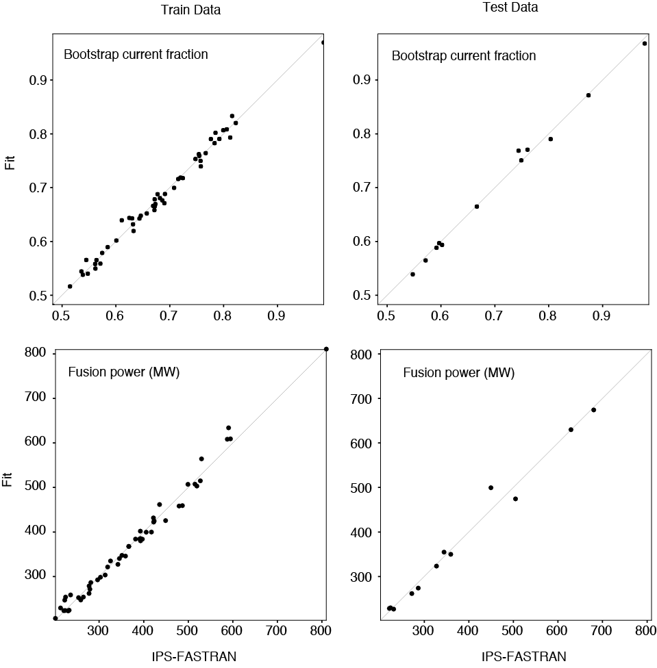
The fitdb.py generates a reduced model using the train dataset (db_train.dat) and evaluates the reduced model accuracy using the test dataset (db_test.dat). As an example, the normalized pressure betaN are parameterized as a function of the scan variables aratio, fgw_ped, nepeak, pinj, and h98. The bootstrap current fraction fbs and the fusion power pfus are parameterized as a function of aratio, fgw_ped, nepeak and betaN

Note

The choice of the independent variables are crucial to the accuracy of the reduced models. Obviousely, the scan variables are good initial try, but not necessarily best represents the system. This topic will appear in many places in the following sections.

fitdb.json

{
"fbs": {
    "model":"linear",
    "scaler_x":"log",
    "scaler_y":"log",
    "variables": [
        "aratio", "fgw_ped", "nepeak", "betan"],
    "parameter": {
    }
},

"pfus": {
    "model":"linear",
    "scaler_x":"log",
    "scaler_y":"log",
    "variables": [
        "aratio", "fgw_ped", "nepeak", "betan"],
    "parameter": {
    }
},

"betan": {
    "model":"linear",
    "scaler_x":"log",
    "scaler_y":"log",
    "variables": [
        "aratio", "pinj", "fgw_ped", "nepeak", "h98"],
    "parameter": {
    }
}
}

See also the Neural Network reduced model example.

fitout.json

The output file fitout.json contains the coefficients of the LL regression.

{
    "fbs": [
        "loglinear",
        {
            "const": 0.18823371506585898,
            "aratio": -0.4430942101868331,
            "fgw_ped": -0.1350619408712145,
            "nepeak": 0.21081006299692615,
            "betan": 1.1310480676370078
        }
    ],
    "pfus": [
        "loglinear",
        {
            "const": 1.64943792579016,
            "aratio": 1.207555937736708,
            "fgw_ped": -0.7255082562105468,
            "nepeak": -0.6954783516280638,
            "betan": 2.939140937783406
        }
    ],
    "betan": [
        "loglinear",
        {
            "const": 0.17639747416067017,
            "aratio": 0.8869343206322062,
            "pinj": 0.37591018633973355,
            "fgw_ped": 0.353477277768723,
            "nepeak": 0.3011398492024075,
            "h98": 1.8843684195879282
        }
    ]
}